Permeability is often estimated with compact physics formulas, but heterogeneous pore networks contain connectivity and topology that a bulk formula cannot represent. A GNN can learn those relationships, but adding a neural model everywhere is not automatically better.
TopoFlow asks a more useful question: when does topology add predictive value? I benchmarked a GraphSAGE model against the Kozeny-Carman baseline across five formations, then exposed the result through a FastAPI application with streaming inference, 3D pore visualization, a cloud sample library, and a methodology dashboard.
- Individual work: graph extraction, GraphSAGE implementation, physics benchmarking, API design, and frontend integration.
- Evidence-first result: GNN wins on heterogeneous Savonnières and Estaillades; the physics baseline remains preferable on simpler regimes.
- Reproducibility: source, benchmark artifacts, model weights, architecture, and setup instructions are public.
GraphSAGE Pipeline — Implementation Detail
Pore network extraction — SNOW2 via PoreSpy
Micro-CT voxel data is segmented and passed through the SNOW2 algorithm to extract pores (nodes) and throats (edges). Node features: equivalent pore radius, coordination number, shape factor. Edge features: throat radius and length.
GraphSAGE — 3 aggregation layers
Mean aggregator, ReLU activation, dropout 0.3. Graph-level readout via global mean pooling. Trained against measured permeability (mD) using MSE loss with Adam optimizer.
PyTorch Geometric · GraphSAGE · global_mean_pool
Regime selector — Cv threshold
The coefficient of variation (Cv) of the pore-size distribution determines which model runs. High Cv (heterogeneous) → GraphSAGE. Low Cv (homogeneous) → Kozeny-Carman physics baseline. Threshold calibrated on formation-level test splits.
Cv = σ(r_pore) / μ(r_pore) > threshold → GNN
A Scientific Pipeline, Not Just an Inference Endpoint
Topology Helps in the Complex Regime
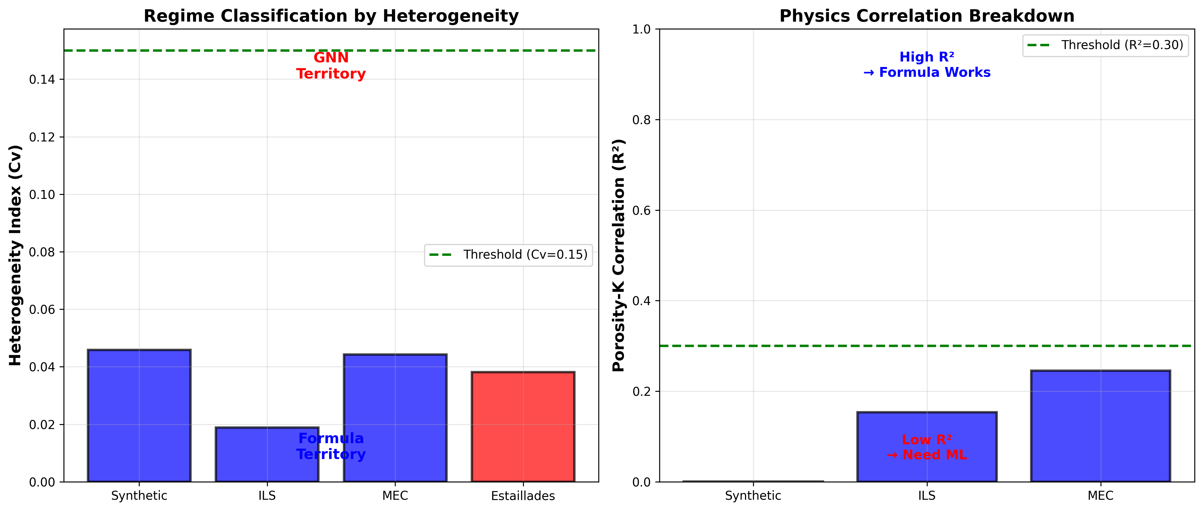
| Formation | Pore-size Cv | Preferred model | Observed result |
|---|---|---|---|
| Savonnières | ~2.5 | GraphSAGE | 46.2% lower MSE |
| Estaillades | 2.80 | GraphSAGE | 28.4% lower MSE |
| MEC Carbonate | 0.85 | Physics | Added model complexity not justified |
| ILS Limestone | 0.52 | Physics | Added model complexity not justified |
| Synthetic | 0.45 | Physics | Added model complexity not justified |
From Scientific Pipeline to Usable Tool
Select or upload a rock volume
The application supports local files and a Supabase-backed sample catalog, with a server-side proxy so cloud credentials stay outside the browser.
Extract and inspect the pore network
Large arrays are downsampled server-side for visualization while the scientific pipeline retains the full representation for graph extraction and inference.
Stream progress through the API
FastAPI exposes prediction and visualization routes, while Server-Sent Events keep the interface responsive during graph construction and model execution.
Return the model and the reason
The result includes permeability, structural statistics, and the selected regime so the user can see why graph learning or physics was used.
Where the Work Became Interesting
GNNs did not win everywhere
A single average score hid a meaningful difference between homogeneous and heterogeneous formations.
Turned failure into a regime rule
Compared per-formation behavior and used pore-size heterogeneity to preserve the simpler physics model where topology added no measurable value.
Scientific arrays were too large for the browser
Rendering full micro-CT volumes made the UI slow and memory-heavy.
Separated inference and visualization grains
The backend keeps the scientific representation for prediction while returning a bounded, deterministic visualization payload to Plotly.js.
Long-running extraction felt broken
Graph extraction can take time before the user sees a result.
Added streaming progress
Server-Sent Events expose pipeline progress without coupling the scientific library to frontend state.